Note
Go to the end to download the full example code.
R=DV and other matrix decompositions
R = DV factorization is a standard tool to compute persistent homology. OAT obtains R=DV factorizations by way of Umatch decompositions. This tutorial shows how to obtain
Umatch decompositions
R=DV factorizations
R=DV factorizations of the anti-transpose of D (for persistent cohomology)
RU=D factorizations
import oat_python as oat

from fractions import Fraction
import matplotlib.pyplot as plt
import numpy as np
import pandas as pd
import plotly.graph_objects as go
from scipy.sparse import csr_matrix
Setup
Define a function to check equality of sparse matrices
def sparse_matrices_equal(A, B):
    """Check if two scipy sparse matrices are equal."""
    # Check shape first
    if A.shape != B.shape:
        return False
    # Subtract and check if all elements are zero
    diff = (A != B).nnz == 0
    return diff
Generate a point cloud
points = oat.point_cloud.sphere_or_slice_spiral(n_points=8, noise_scale=0.07, random_seed=0)
Plot the point cloud
trace               =   go.Scatter3d(x=points[:,0],y=points[:,1],z=points[:,2], mode="markers", marker=dict(opacity=1, size=4, color=points[:,2], colorscale="Aggrnyl"))
fig                 =   go.Figure(data=trace)
fig.update_layout(title=dict(text="Point cloud"), height=800,width=850)
fig
Compute persistent homology
We compute persistent homology by factoring the boundary matrix. The following cell generates a sparse distance matrix and feeds it to the persistent homology solver. The result is a decomposition boundary matrix. We will extract information from this matrix in the following cells.
Prepare a dissimilarity matrix
# Calculate the minimum enclosing radius. There is a theorem that states all
# homology vanishes above this filtration parameter, so we can exclude
# simplices whose diameter is larger than this value from the complex.
enclosing_radius        =   oat.dissimilarity.enclosing_radius_for_points(points)

# Format the dissimilarity matrix.
# This produces a dissimilarity matrix where all values over
# enclosing_radius + 0.0000000001 are removed. Adding 0.0000000001 avoids
# problems due to numerical error.
dissimilarity_matrix    =   oat.dissimilarity.sparse_matrix_for_points(
                                points                   =   points,
                                max_dissimilarity        =   enclosing_radius + 0.00000000001,
                            )
Create and decompose the boundary matrix
decomposition           =   oat.core.vietoris_rips.BoundaryMatrixDecomposition(
                                dissimilarity_matrix    =   dissimilarity_matrix,
                            )
Compute the boundary of a chain
chain                   =   pd.DataFrame([
                                { "simplex":(0,1,2), "coefficient":Fraction(1, 1)  },
                                { "simplex":(4,5,6), "coefficient":Fraction(1, 1)  },
                            ])
boundary_matrix         =   decomposition.boundary_matrix_oracle()
boundary                =   boundary_matrix.boundary_for_chain( chain )
oat.plot.display_dataframes_side_by_side(
    chain, boundary,
    titles=  ["Chain", "Boundary for this chain"]
)
Sort the simplices in the boundary by lexicographic order
boundary.sort_values(inplace=True, by="simplex")
boundary
Compute a coboundary
cochain                 =   pd.DataFrame([
                                { "simplex":(0,1), "coefficient":Fraction(1, 1)  },
                            ])
coboundary              =   boundary_matrix.coboundary_for_cochain( cochain )
oat.plot.display_dataframes_side_by_side(
    cochain, coboundary,
    titles=  ["Cochain", "Coboundary for this cochain"]
)
A boundary matrix
D                       =   decomposition.boundary_matrix_as_csr()

plt.figure(figsize=(6, 6))
plt.spy(D, markersize=2, color="orange")
plt.title("D (boundary matrix)", y=-0.18)  # Move title to the bottom
plt.tight_layout()
plt.show()
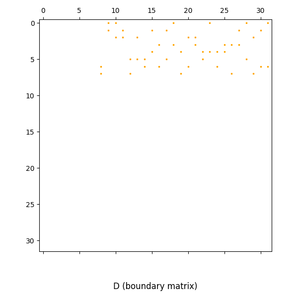
The simplex corresponding to each row and column of the boundary matrix can be obtained as follows.
This list includes all simplices of dimension <= max_homology_dimension, and all negative simplices of dimension max_homology_dimension + 1.
Simplices are sorted first by dimension, then by filtration value, then lexicographically.
decomposition.boundary_matrix_indices_df()
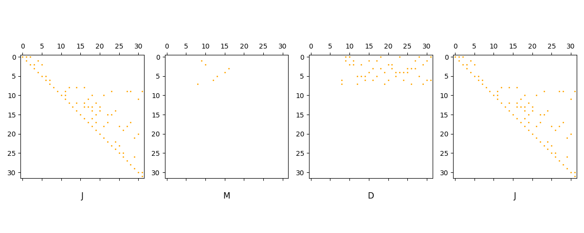
A differential Umatch decomposition
A differential Umatch decomposition is a tuple of matrices \((J,M,D,J)\), where
\(D\) is a boundary matrix
\(J\) is a square upper triangular matrix with ones on the diagonal
\(M\) is a generalized matching matrix
See Differential Umatch Decomposition for definitions and background. Umatch decompositions can be used to obtain
\(R=DV\) decompositions by setting \(V=J\) and \(R=DJ\)
\(RU=D\) decompositions by setting \(U = J^{-1}\).
\(R=WD\) decompositions by setting \(W=J^{-1}\) and \(R=J^{-1}D\)
this is the calculation used to obtain persistent cohomology
it is commonly described as \(R=DV\) decomposition of the antitranspose \(D^\perp\)
\(YR=D\) decompositions by setting \(Y = J\).
D                       =   decomposition.boundary_matrix_as_csr()
J                       =   decomposition.differential_comb_as_csr()
M                       =   decomposition.generalized_matching_matrix_as_csr()

D.data                  =   D.data.astype(float)
J.data                  =   J.data.astype(float)
M.data                  =   M.data.astype(float)


#   plot sparsity patterns
fig, axs = plt.subplots(1,4)
fig.set_figwidth(12)


axs[0].spy(J,   precision=0, marker=None, markersize=1, color="orange", aspect='equal', origin='upper')
axs[1].spy(M,   precision=0, marker=None, markersize=1, color="orange", aspect='equal', origin='upper')
axs[2].spy(D,   precision=0, marker=None, markersize=1, color="orange", aspect='equal', origin='upper')
axs[3].spy(J,   precision=0, marker=None, markersize=1, color="orange", aspect='equal', origin='upper')
axs[0].set_title("J", y=-0.2)
axs[1].set_title("M", y=-0.2)
axs[2].set_title("D", y=-0.2)
axs[3].set_title("J", y=-0.2)
plt.tight_layout()
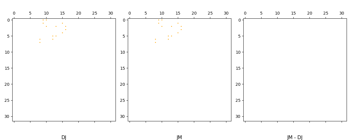
Verify that that JM = DJ
sparse_matrices_equal( J@M, D@J )
True
Visualize the difference JM - DJ, just to be thorough:
fig, axs = plt.subplots(1,3)
fig.set_figwidth(12)


axs[0].spy(D @ J,   precision=0, marker=None, markersize=1, color="orange", aspect='equal', origin='upper')
axs[1].spy(J @ M,       precision=0, marker=None, markersize=1, color="orange", aspect='equal', origin='upper')
axs[2].spy( (J@M) - (D@J),       precision=0, marker=None, markersize=1, color="orange", aspect='equal', origin='upper')
axs[0].set_title("DJ", y=-0.2)
axs[1].set_title("JM", y=-0.2)
axs[2].set_title("JM - DJ", y=-0.2)
plt.tight_layout()
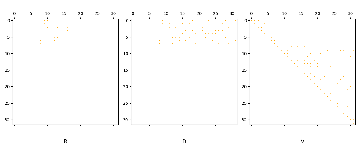
# An R = DV decomposition
As noted above, Umatch decompositions can be used to obtain \(R=DV\) decompositions by setting \(V=J\) and \(R=DJ\).
Scipy has limited functionality for coefficients of type Fraction, so convert to float
J.data              =   J.data.astype(float)
D.data              =   D.data.astype(float)

#   plot sparsity patterns
fig, axs = plt.subplots(1,3)
fig.set_figwidth(12)


axs[0].spy(D @ J,   precision=0, marker=None, markersize=1, color="orange", aspect='equal', origin='upper')
axs[1].spy(D,       precision=0, marker=None, markersize=1, color="orange", aspect='equal', origin='upper')
axs[2].spy(J,       precision=0, marker=None, markersize=1, color="orange", aspect='equal', origin='upper')
axs[0].set_title("R", y=-0.2)
axs[1].set_title("D", y=-0.2)
axs[2].set_title("V", y=-0.2)
plt.tight_layout()
Verify that R: = DJ is in fact reducted
def bottom_nonzero_rows_are_unique(A: csr_matrix):
    """
    Returns True if, for all distinct nonzero columns i and j of A,
    the bottom (last) nonzero element of each column occurs in a different row.
    """
    # Find nonzero columns
    nonzero_cols = np.flatnonzero(A.getnnz(axis=0))
    # For each nonzero column, find the row index of the bottom nonzero element
    bottom_rows = []
    for col in nonzero_cols:
        col_data = A[:, col].tocoo()
        if col_data.row.size > 0:
            bottom_rows.append(col_data.row.max())
    # Check if all bottom rows are unique
    return len(bottom_rows) == len(set(bottom_rows))

# Example usage:
bottom_nonzero_rows_are_unique(D @J)
True
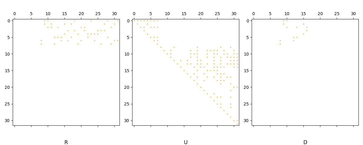
An RU = D decomposition
As noted above, Umatch decompositions can be used to obtain \(RU = D\) decompositions by setting \(U = J^{-1}\) and \(R = DJ\).
Jinv                =   decomposition.differential_comb_inverse_as_csr()

#   Scipy has limited functionality for coefficients of type Fraction, so convert to float
Jinv.data           =   Jinv.data.astype(float)
D.data              =   D.data.astype(float)

#   plot sparsity patterns
fig, axs = plt.subplots(1,3)
fig.set_figwidth(12)


axs[0].spy((D @ J) @ Jinv,   precision=0, marker=None, markersize=1, color="orange", aspect='equal', origin='upper')
axs[1].spy(Jinv,       precision=0, marker=None, markersize=1, color="orange", aspect='equal', origin='upper')
axs[2].spy(D @ J,       precision=0, marker=None, markersize=1, color="orange", aspect='equal', origin='upper')
axs[0].set_title("R", y=-0.2)
axs[1].set_title("U", y=-0.2)
axs[2].set_title("D", y=-0.2)
plt.tight_layout()
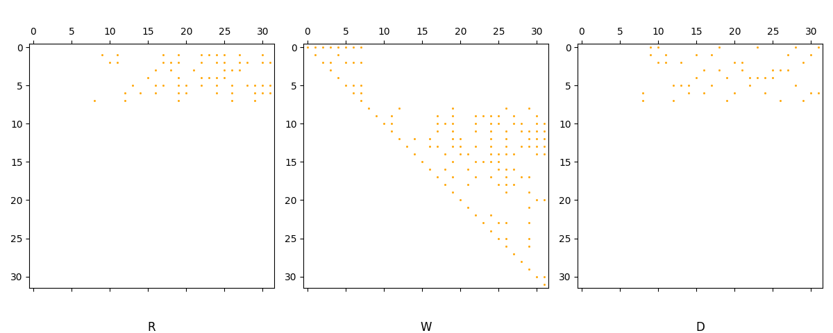
An \(R=DV\) decomposition of \(D^\perp\) (persistent cohomology)
This is equivalent to a matrix equation R = WD where W is invertible and upper triangular, and where R is reduced in the sense that the leading entry of every nonzero row occurs in a distinct column.
fig, axs = plt.subplots(1,3)
fig.set_figwidth(12)

axs[0].spy(Jinv @ D,   precision=0, marker=None, markersize=1, color="orange", aspect='equal', origin='upper')
axs[1].spy(Jinv,       precision=0, marker=None, markersize=1, color="orange", aspect='equal', origin='upper')
axs[2].spy(D,       precision=0, marker=None, markersize=1, color="orange", aspect='equal', origin='upper')
axs[0].set_title("R", y=-0.2)
axs[1].set_title("W", y=-0.2)
axs[2].set_title("D", y=-0.2)
plt.tight_layout()
Verify that \(R\) is reduced in the correct sense.
def leading_nonzero_cols_are_unique(A: csr_matrix):
    """
    Returns True if, for all distinct nonzero rows i and j of A,
    the leading (first) nonzero element of each row occurs in a different column.
    """
    # Find nonzero rows
    nonzero_rows = np.flatnonzero(A.getnnz(axis=1))
    # For each nonzero row, find the column index of the first nonzero element
    leading_cols = []
    for row in nonzero_rows:
        row_data = A[row, :].tocoo()
        if row_data.col.size > 0:
            leading_cols.append(row_data.col.min())
    # Check if all leading columns are unique
    return len(leading_cols) == len(set(leading_cols))

# Example usage:
leading_nonzero_cols_are_unique( Jinv @ D)
True
Total running time of the script: (0 minutes 0.893 seconds)